| YOLOX解读 | 您所在的位置:网站首页 › anchor怎么读 › YOLOX解读 |
YOLOX解读
|
转载自:https://blog.csdn.net/weixin_46142822/article/details/124086230 论文:YOLOX: Exceeding YOLO Series in 2021 论文链接:https://arxiv.org/pdf/2107.08430.pdf 代码链接:https://github.com/Megvii-BaseDetection/YOLOX. 文章目录 1 为什么提出YOLOX 2 YOLOX 网络架构 3 YOLOX 实施细节 3.1 backbone 3.2 neck 3.3 Head 3.3.1 Decoupled Head 3.3.2 Anchor-free 3.4 如何计算Loss 3.5 如何分配标签? 4 YOLOX 性能效果 5 总结 1 为什么提出YOLOX 目标检测分为Anchor Based和Anchor Free两种方式。 在Yolov3、Yolov4、Yolov5中,通常都是采用 Anchor Based的方式,来提取目标框。 Yolox 将 Anchor free 的方式引入到Yolo系列中,使用anchor free方法有如下好处: (1) 降低了计算量,不涉及IoU计算,另外产生的预测框数量也更少。 假设 feature map的尺度为 80 × 80 ,anchor based 方法在Feature Map上,每个单元格一般设置三个不同尺寸大小的锚框,因此产生 3 × 80 × 80 = 19200个预测框。而使用anchor free的方法,则仅产生 80 × 80 = 6400个预测框,降低了计算量。 (2) 缓解了正负样本不平衡问题 anchor free方法的预测框只有anchor based方法的1/3,而预测框中大部分是负样本,因此anchor free方法可以减少负样本数,进一步缓解了正负样本不平衡问题。 (3) 避免了anchor的调参 anchor based方法的anchor box的尺度是一个超参数,不同的超参设置会影响模型性能,anchor free方法避免了这一点。 2 YOLOX 网络架构YOLOX是在YOLOV3基础上做的改进,主体网络框架如下: 输入端 :表示输入的图片,采用的数据增强方式:RandomHorizontalFlip、ColorJitter、多尺度增强 BackBone :用来提取图片特征,采用 Darknet53。 Neck:用于特征融合,采用 PAFPN。 Head: 用来结果预测,主要亮点是采用Decoupled Head、Anchor-free、Multi positives 3 YOLOX 实施细节 3.1 backbone self.backbone = CSPDarknet(depth, width, depthwise=depthwise, act=act) 实例化backbone,采用的是 darknet53。 darknet53具体结构参考下面的图片,左侧是 darknet-53 结构图,右侧是对左侧中的 “convolutional” 层 和 “residual” 层的细节展示。
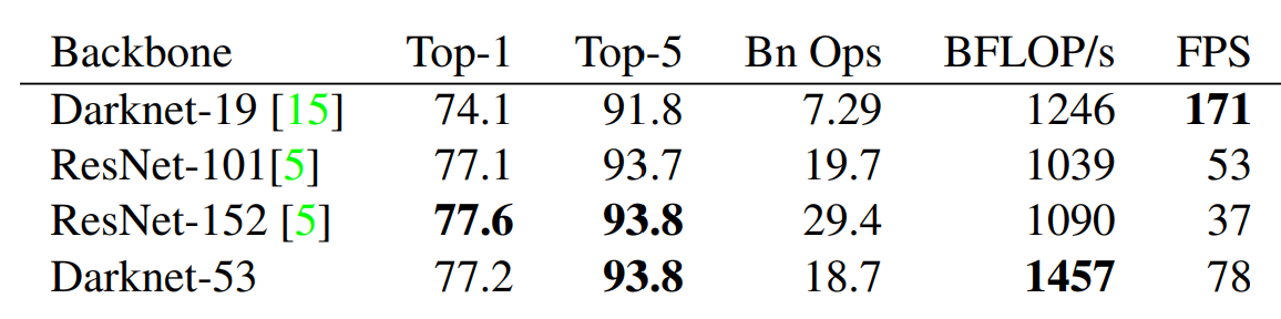
为什么使用 darknet-53 backbone? darknet-53 的性能接近 ResNet-152,但是 FPS 要高一倍。
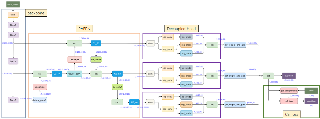
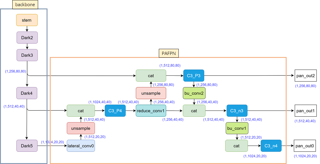
out_features = self.backbone(input) backbone的输入input为一个batch的图片 (B,C,H,W),其中B为batchsize,C为图片的channel数,如果是RGB图片,则C=3,H,W分别是图片的高宽。 假设batchsize为1,宽高分别为640,640,则 demo input可以表示为: torch.randn((1,3,640,640))。 out_features的输出为3个特征层(分别为’dark3’,‘dark4’,‘dark5’)组成的字典,各特征层的shape如下: {'dark3':(1,256,80,80), 'dark4':(1,512,40,40), 'dark5':(1,1024,20,20)} 3.2 neck features = [out_features[f] for f in self.in_features] [x2, x1, x0] = features # x0:(1,1024,20,20) # x1:(1,512,40,40) # x2:(1,256,80,80) fpn_out0 = self.lateral_conv0(x0) # (1,512,20,20) f_out0 = self.upsample(fpn_out0) # (1,512,40,40) f_out0 = torch.cat([f_out0, x1], 1) # (1,1024,40,40) f_out0 = self.C3_p4(f_out0) # (1,512,40,40) fpn_out1 = self.reduce_conv1(f_out0) # (1,256,40,40) f_out1 = self.upsample(fpn_out1) # (1,256,80,80) f_out1 = torch.cat([f_out1, x2], 1) # (1,512,80,80) pan_out2 = self.C3_p3(f_out1) # (1,256,80,80) p_out1 = self.bu_conv2(pan_out2) # (1,256,40,40) p_out1 = torch.cat([p_out1, fpn_out1], 1) # (1,512,40,40) pan_out1 = self.C3_n3(p_out1) # (1,512,40,40) p_out0 = self.bu_conv1(pan_out1) # (1,512,20,20) p_out0 = torch.cat([p_out0, fpn_out0], 1) # (1,1024,20,20) pan_out0 = self.C3_n4(p_out0) # (1,1024,20,20) outputs = (pan_out2, pan_out1, pan_out0)
在Neck结构中,Yolox采用PAFPN的结构进行融合。如下图所示,将高层的特征信息,先通过上采样的方式进行传递融合,再通过下采样融合方式得到预测的特征图,最终输出3个特征层组成的元组结果,各特征层的shape如下: ((1,256,80,80),(1,512,40,40),(1,1024,20,20))
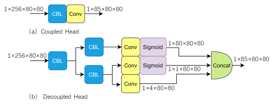
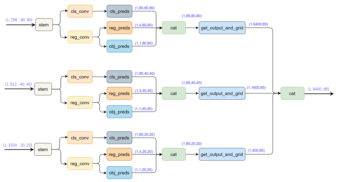
3.3 Head 为了便于理解,我们假定图片上有3个目标框,即3个groundtruth,再假定项目有80个检测类别,则head 输出维度为85 (80+1+4),其中80为类别分数,为1为目标分数,4为bbox的坐标。 3.3.1 Decoupled Head之前yolo 系列都是使用coupled head, yolox使用decoupled head。 coupled head 和 decoupled head 有什么差异? 当使用coupled head时,网络直接输出shape (1,85,80,80); 如果使用 decoupled head,网络会分成回归分支和分类分支,最后再汇总在一起,得到shape同样为 (1,85,80,80)。
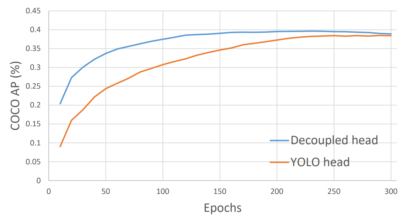
为什么用decoupled head? 如果使用coupled head,输出channel将分类任务和回归任务放在一起,这2个任务存在冲突性。(论文中说有冲突性,但是没有理解为什么存在冲突,我考虑的是从损失函数角度存在冲突) 通过实验发现替换为Decoupled Head后,不仅是模型精度上会提高,同时 网络的收敛速度也加快了,使用Decoupled Head的表达能力更好。 Yolo Head和 Decoupled Head 的对比曲线如下:
3.3.2 Anchor-free 有2种经典的anchor free目标检测模型,分别为FCOS和CenterNet,参考如下博客: 目标检测: 一文读懂 CenterNet (CVPR 2019)_大林兄的博客-CSDN博客 目标检测: 一文读懂 FCOS (CVPR 2019)_大林兄的博客-CSDN博客 如果只指定一个点作为positive,很多其他高质量的预测如果不纳入来计算loss,这不利于训练,(批注:该行所说的问题是:在anchor-base中,用于训练的正样本只有一个,而在anchor-free当中,用于训练的正样本会有很多) Yolox使用FCOS中的center sampling方法,将目标中心3x3的区域内的像素点都作为 target,这在Yolox论文中称为 multi positives。 3.4 如何计算Loss进行Loss 计算前,需要将不同特征层的输出预测框映射回原图。通过get_output_and_grid函数实现 ,核心代码如下: # 以下的注释中,尺寸不正确,要注意区分很多地方的尺寸都是2,比如wh,xyhsize, wsize = output.shape[-2:] # hsize:80, wsize:80 yv, xv = meshgrid([torch.arange(hsize), torch.arange(wsize)]) #yv, xv shape: (1,85,80,80),(1,85,80,80) grid = torch.stack((xv, yv), 2).view(1, 1, hsize, wsize,2).type(dtype) #grid shape: (1,1,85,80,80) grid = grid.view(1, -1, 2) #grid shape: (1,6400,2) output[..., :2] = (output[..., :2] + grid) * stride # output[..., :2]是anchor中心店的offset #output shape: (1,6400,85) output[..., 2:4] = torch.exp(output[..., 2:4]) * stride #output[..., 2:4]是wh #output shape: (1,6400,85)
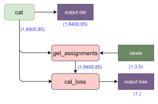
代码中前4行是生成gird的坐标,第5行则计算bbox中心坐标。 因为head关于bbox的输出位置是相对grid的距离,所以映射回原图需要加上grid坐标。 宽高尺寸为正数,所以对output的宽高先做指数运算,再乘上stride,得到原图尺度下的宽高。 最后将3个特征图上的预测框结果合并,得到所有的预测框结果(目标检测最后计算损失都是将所有尺度的框映射原图后汇总,然后再筛选正负样本,最后计算loss),输出shape为(1,8400,85)。
得到预测结果之后,如果是推断,只要输出output det即可。 如果是训练,需要通过函数 get_assignments 先得到 8400个预测框的target,即标签分配,随后再进行loss计算。
如果得到了 target,loss计算公式如下: l o s s ==λ⋅lossreg+lossobj+losscls+lossl1 代码实现如下: loss_iou = (self.iou_loss(bbox_preds.view(-1, 4)[fg_masks], reg_targets)).sum() / num_fg loss_obj = (self.bcewithlog_loss(obj_preds.view(-1, 1), obj_targets)).sum() / num_fg loss_cls = (self.bcewithlog_loss(cls_preds.view(-1, self.num_classes)[fg_masks], cls_targets)).sum() / num_fg if self.use_l1: loss_l1 = (self.l1_loss(origin_preds.view(-1, 4)[fg_masks], l1_targets)). sum() / num_fg else: loss_l1 = 0.0 reg_weight = 5.0 loss = reg_weight * loss_iou + loss_obj + loss_cls + loss_l1 3.5 如何分配标签?经过 3个head的输出,一共有8400个预测框,这8400个预测框的标签是什么? 这8400个预测框绝大部分是负样本,只有少数是正样本,直接对8400个预测框做精确的标签分配,计算量较大。 yolox分配标签过程分为2步:(1) 粗筛选;(2)simOTA 精确分配标签 step1:粗筛选 筛选出潜在包含正样本的预测框,参见代码: get_in_boxes_info 如果 anchor bbox 中心落在 groundtruth bbox或 fixed bbox,则被选中为候选正样本。 判断 anchor bbox 中心是否在 groundtruth bbox step1:计算groundtruth的左上角、右下角坐标 groundtruth的 gt_bboxes_per_image为:[x_center,y_center,w,h]。 可以根据此信息可以计算出groundtruth 的左上角、右下角坐标: ## 方法1(groundtruth bbox): l,r,t,b gt_bboxes_per_image_l = ( (gt_bboxes_per_image[:, 0] - 0.5 * gt_bboxes_per_image[:, 2]) .unsqueeze(1) .repeat(1, total_num_anchors) ) # shape:(3,8400) gt_bboxes_per_image_r = ( (gt_bboxes_per_image[:, 0] + 0.5 * gt_bboxes_per_image[:, 2]) .unsqueeze(1) .repeat(1, total_num_anchors) ) # shape:(3,8400) gt_bboxes_per_image_t = ( (gt_bboxes_per_image[:, 1] - 0.5 * gt_bboxes_per_image[:, 3]) .unsqueeze(1) .repeat(1, total_num_anchors) ) # shape:(3,8400) gt_bboxes_per_image_b = ( (gt_bboxes_per_image[:, 1] + 0.5 * gt_bboxes_per_image[:, 3]) .unsqueeze(1) .repeat(1, total_num_anchors) ) # shape:(3,8400)
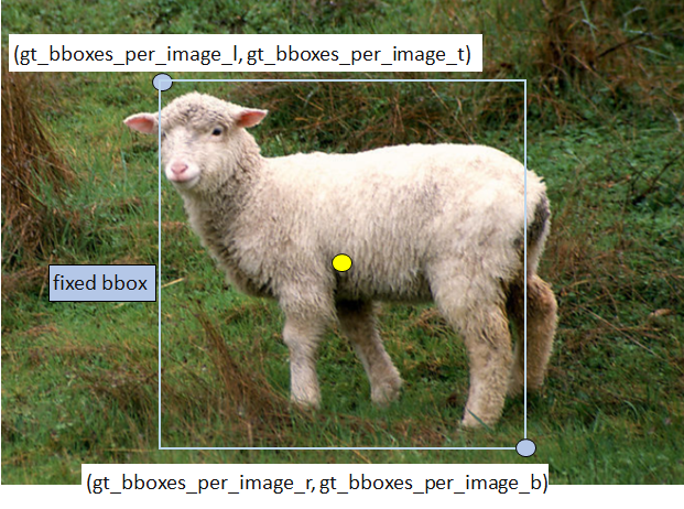
step2:判断anchor bbox 中心是否落在groudtruth边框范围内 前4行代码计算锚框中心点(x_center,y_center),和标注框左上角(gt_l,gt_t),右下角(gt_r,gt_b)两个角点的相应距离。 b_l = x_centers_per_image - gt_bboxes_per_image_l # shape:(3,8400) b_r = gt_bboxes_per_image_r - x_centers_per_image # shape:(3,8400) b_t = y_centers_per_image - gt_bboxes_per_image_t # shape:(3,8400) b_b = gt_bboxes_per_image_b - y_centers_per_image # shape:(3,8400) bbox_deltas = torch.stack([b_l, b_t, b_r, b_b], 2) # shape:(3,8400,4) is_in_boxes = bbox_deltas.min(dim=-1).values > 0.0 # shape:(3,8400) is_in_boxes_all = is_in_boxes.sum(dim=0) > 0 # shape:(8400,)第5行将四个值叠加之后,通过第六行,判断是否都大于0? 就可以将落在groundtruth矩形范围内的所有anchors,都提取出来了。 因为ancor box的中心点,只有落在矩形范围内,这时的b_l,b_r,b_t,b_b都大于0。 判断anchor bbox 中心是否在 fixed bbox 以groundtruth的中心点为中心,在特征层尺度上做 5 × 5 的正方形。 如果图片的尺寸为 640 × 640,且当前特征图的尺度为 80 × 80 ,则此时stride为 8, 将 5 × 5 的正方形映射回原图,fixed bbox 尺寸为 400 × 400 。 所以如果 ancor box的中心点落在 fixed bbox范围内,也将被选中。 ## 方法2(fixed bbox): l,r,t,b center_radius = 2.5 gt_bboxes_per_image_l = ( gt_bboxes_per_image[:, 0]).unsqueeze(1).repeat( 1, total_num_anchors ) - center_radius * expanded_strides_per_image.unsqueeze(0) gt_bboxes_per_image_r = ( gt_bboxes_per_image[:, 0]).unsqueeze(1).repeat( 1, total_num_anchors ) + center_radius * expanded_strides_per_image.unsqueeze(0) gt_bboxes_per_image_t = ( gt_bboxes_per_image[:, 1]).unsqueeze(1).repeat( 1, total_num_anchors ) - center_radius * expanded_strides_per_image.unsqueeze(0) gt_bboxes_per_image_b = ( gt_bboxes_per_image[:, 1]).unsqueeze(1).repeat( 1, total_num_anchors ) + center_radius * expanded_strides_per_image.unsqueeze(0)
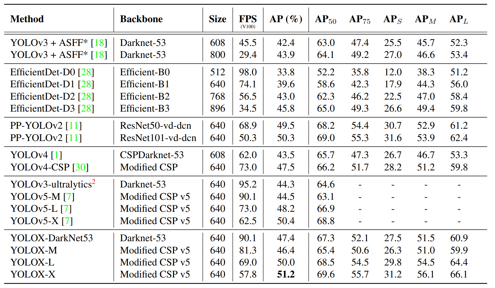
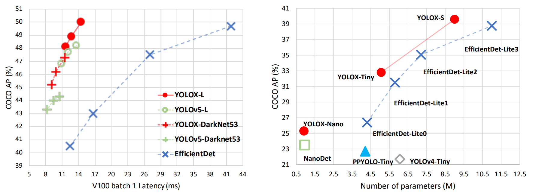
未选中的预测框为负样本,直接打上负样本标签。 (2) step2:simOTA 经过粗筛选,假设筛选出1000个预测框为潜在正样本,这1000个预测框并不是都作为正样本分配标签,而是需要进一步做标签分配,yolox使用simOTA方法,该方法的详细介绍参见博客: 目标检测: 一文读懂 OTA 标签分配_大林兄的博客-CSDN博客 4 YOLOX 性能效果YOLOX的性能超越了YOLOV5,YOLOX-X的AP值达到了51.2,超过YOLOV5-X 0.8个百分点,此外模型推理速度和参数量都具有比较大的优势。
5 总结 YOLOX做出了如下贡献: (1) 将 anchor free 方法引入到YOLO系列,性能超越了基于anchor based方法的yolov5; (2) 采用了 decoupled head、simOTA等方法,值得借鉴。 |


【本文地址】