深度学习 |
您所在的位置:网站首页 › 如何识别花的种类 › 深度学习 |
深度学习
|
深度学习-tensorflow对花的品种进行分类
这里会展示如何对花的图像进行分类。它使用keras创建一个图像分类器。顺序模型,并使用预处理.image_dataset_from_directory加载数据。 主要的流程就是加载数据集。识别过拟合并应用技术来减轻它,包括数据扩充和Dropout。 基本的机器学习流程:检查和理解数据 构建输入管道 构建模型 训练模型 测试模型 改进模型并重复此过程 导入TensorFlow和其他库 import matplotlib.pyplot as plt import numpy as np import os import PIL import tensorflow as tf from tensorflow import keras from tensorflow.keras import layers from tensorflow.keras.models import Sequential 下载数据下载并浏览数据集 本教程使用了大约3700张鲜花照片的数据集。数据集包含5个子目录,每个类一个: import pathlib dataset_url = "https://storage.googleapis.com/download.tensorflow.org/example_images/flower_photos.tgz" data_dir = tf.keras.utils.get_file('flower_photos', origin=dataset_url, untar=True) data_dir = pathlib.Path(data_dir)下载之后,您现在应该有一个可用的数据集副本。总共有3670张图片: image_count = len(list(data_dir.glob('*/*.jpg'))) print(image_count)如果执行上面的程序后,就会得到3670 接下来我们可以看下我们下载的数据里面有什么图片,我们任意选几张来看下。 roses = list(data_dir.glob('roses/*')) PIL.Image.open(str(roses[0]))
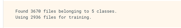
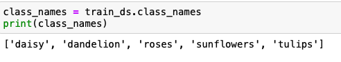
负载使用keras.preprocessing 使用有用的image_dataset_from_directory实用程序将这些图像从磁盘上加载下来。这将把从磁盘上的图像目录到一个tf.data.Dataset只需几行代码。如果愿意,还可以通过访问加载图像教程从头编写自己的数据加载代码。 创建一个数据集为加载器定义一些参数: batch_size = 32 img_height = 180 img_width = 180在开发模型时使用验证分割是一个很好的实践。我们使用80%的图像进行训练,20%进行验证。 train_ds = tf.keras.preprocessing.image_dataset_from_directory( data_dir, validation_split=0.2, subset="training", seed=123, image_size=(img_height, img_width), batch_size=batch_size)你可以看到跑出这样子的结果 Found 3670 files belonging to 5 classes. Using 734 files for validation. 可以在这些数据集中的class_names属性中找到类名。这些按字母顺序对应目录名。 class_names = train_ds.class_names print(class_names)
以下是来自训练数据集的前9张图片。 import matplotlib.pyplot as plt plt.figure(figsize=(10, 10)) for images, labels in train_ds.take(1): for i in range(9): ax = plt.subplot(3, 3, i + 1) plt.imshow(images[i].numpy().astype("uint8")) plt.title(class_names[labels[i]]) plt.axis("off")
(32, 180, 180, 3) (32,) image_batch是一个形状张量(32,180,180,3)。这是一批32张形状为180x180x3的图像(最后一个维度是彩色通道RGB)。label_batch是一个形状(32,)的张量,这些是32幅图像对应的标签。 可以对image_batch和labels_batch张量调用.numpy()将它们转换为numpy.ndarray。 为性能配置数据集 让我们确保使用缓冲预取,这样就可以在不阻塞I/O的情况下从磁盘生成数据。这是加载数据时应该使用的两个重要方法。 AUTOTUNE = tf.data.AUTOTUNE train_ds = train_ds.cache().shuffle(1000).prefetch(buffer_size=AUTOTUNE) val_ds = val_ds.cache().prefetch(buffer_size=AUTOTUNE) 标准化的数据RGB通道值在[0,255]范围内。这对于神经网络来说并不理想;通常,应该设法使输入值小一些。在这里,使用一个rescale层来标准化[0,1]范围内的值。 normalization_layer = layers.experimental.preprocessing.Rescaling(1./255) normalized_ds = train_ds.map(lambda x, y: (normalization_layer(x), y)) image_batch, labels_batch = next(iter(normalized_ds)) first_image = image_batch[0] # Notice the pixels values are now in `[0,1]`. print(np.min(first_image), np.max(first_image))可以在模型定义中包含该层,这可以简化部署。我们用第二种方法。 创建模型该模型由三个卷积块组成,每个卷积块中有一个最大池层。有一个完全连接的层,上面有128个单元,由一个relu激活功能激活。这个模型还没有进行高精度的调整。 num_classes = 5 model = Sequential([ layers.experimental.preprocessing.Rescaling(1./255, input_shape=(img_height, img_width, 3)), layers.Conv2D(16, 3, padding='same', activation='relu'), layers.MaxPooling2D(), layers.Conv2D(32, 3, padding='same', activation='relu'), layers.MaxPooling2D(), layers.Conv2D(64, 3, padding='same', activation='relu'), layers.MaxPooling2D(), layers.Flatten(), layers.Dense(128, activation='relu'), layers.Dense(num_classes) ]) 编译模型对于本教程,选择优化器。亚当优化和损失。SparseCategoricalCrossentropy损失函数。要查看每个培训阶段的培训和验证准确性,请传递metrics参数。 model.compile(optimizer='adam', loss=tf.keras.losses.SparseCategoricalCrossentropy(from_logits=True), metrics=['accuracy']) 模型的总结使用模型的汇总方法查看网络的所有层: model.summary()
训练模型 epochs=10 history = model.fit( train_ds, validation_data=val_ds, epochs=epochs )
在培训和验证集上创建损失和准确性图。 acc = history.history['accuracy'] val_acc = history.history['val_accuracy'] loss = history.history['loss'] val_loss = history.history['val_loss'] epochs_range = range(epochs) plt.figure(figsize=(8, 8)) plt.subplot(1, 2, 1) plt.plot(epochs_range, acc, label='Training Accuracy') plt.plot(epochs_range, val_acc, label='Validation Accuracy') plt.legend(loc='lower right') plt.title('Training and Validation Accuracy') plt.subplot(1, 2, 2) plt.plot(epochs_range, loss, label='Training Loss') plt.plot(epochs_range, val_loss, label='Validation Loss') plt.legend(loc='upper right') plt.title('Training and Validation Loss') plt.show()
从图中可以看到,训练精度和验证精度相差很大,模型在验证集上仅实现了约60%的准确性。 看看哪里出了问题,尝试提高模型的整体性能。 过度拟合在上面的图中,训练精度随时间线性增加,而验证精度在训练过程中停滞在60%左右。此外,训练和验证准确性之间的差异是明显的——这是过度拟合的迹象。 当训练样本数量很少时,模型有时会从训练样本的噪声或不需要的细节中学习,这在一定程度上会对模型在新样本上的性能产生负面影响。这种现象被称为过拟合。这意味着模型在新的数据集中泛化时会有困难。 在训练过程中有多种方法可以对抗过拟合。在本教程中,将使用数据增强并将Dropout添加到您的模型中。 数据增加 过拟合通常发生在只有少量训练例子的情况下。数据增强采用的方法是从现有的例子中生成额外的训练数据,通过使用随机变换来增强它们,产生看起来可信的图像。这有助于向数据的更多方面公开模型,并更好地一般化。 使用来自tf.keras.layers.experimental.preprocessing的层来实现数据增强。它们可以像其他层一样被包含在你的模型中,并在GPU上运行。 data_augmentation = keras.Sequential( [ layers.experimental.preprocessing.RandomFlip("horizontal", input_shape=(img_height, img_width, 3)), layers.experimental.preprocessing.RandomRotation(0.1), layers.experimental.preprocessing.RandomZoom(0.1), ] )让我们通过多次对同一幅图像应用数据增强来可视化几个增强示例: plt.figure(figsize=(10, 10)) for images, _ in train_ds.take(1): for i in range(9): augmented_images = data_augmentation(images) ax = plt.subplot(3, 3, i + 1) plt.imshow(augmented_images[0].numpy().astype("uint8")) plt.axis("off")
应用数据增强和Dropout后,过拟合减少,训练和验证精度更接近。 acc = history.history['accuracy'] val_acc = history.history['val_accuracy'] loss = history.history['loss'] val_loss = history.history['val_loss'] epochs_range = range(epochs) plt.figure(figsize=(8, 8)) plt.subplot(1, 2, 1) plt.plot(epochs_range, acc, label='Training Accuracy') plt.plot(epochs_range, val_acc, label='Validation Accuracy') plt.legend(loc='lower right') plt.title('Training and Validation Accuracy') plt.subplot(1, 2, 2) plt.plot(epochs_range, loss, label='Training Loss') plt.plot(epochs_range, val_loss, label='Validation Loss') plt.legend(loc='upper right') plt.title('Training and Validation Loss') plt.show()
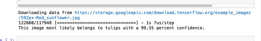
最后,让我们使用我们的模型来分类没有包含在训练或验证集中的图像。 sunflower_url = "https://storage.googleapis.com/download.tensorflow.org/example_images/592px-Red_sunflower.jpg" sunflower_path = tf.keras.utils.get_file('Red_sunflower', origin=sunflower_url) img = keras.preprocessing.image.load_img( sunflower_path, target_size=(img_height, img_width) ) img_array = keras.preprocessing.image.img_to_array(img) img_array = tf.expand_dims(img_array, 0) # Create a batch predictions = model.predict(img_array) score = tf.nn.softmax(predictions[0]) print( "This image most likely belongs to {} with a {:.2f} percent confidence." .format(class_names[np.argmax(score)], 100 * np.max(score)) )
|


 将通过将这些数据集传递给模型来训练模型。一会儿就好

 稍后将使用数据增强来训练模型。 另一种减少过拟合的技术是在网络中引入Dropout,这是一种正则化的形式。 当将Dropout应用到一个层时,它会在训练过程中从该层随机退出一些输出单位(通过将激活设置为零)。Dropout以一个小数作为输入值,形式有0.1、0.2、0.4等。这意味着从应用层中随机去掉10%、20%或40%的输出单元。 让我们用层创建一个新的神经网络。退出,然后用增强图像训练它。
【本文地址】
今日新闻 |
点击排行 |
|
推荐新闻 |
图片新闻 |
|
专题文章 |