| 50种Python论文绘图合集,从入门到精通含代码 | 您所在的位置:网站首页 › python医学科研中能做什么 › 50种Python论文绘图合集,从入门到精通含代码 |
50种Python论文绘图合集,从入门到精通含代码
|
50种Python论文绘图合集,从入门到精通含代码
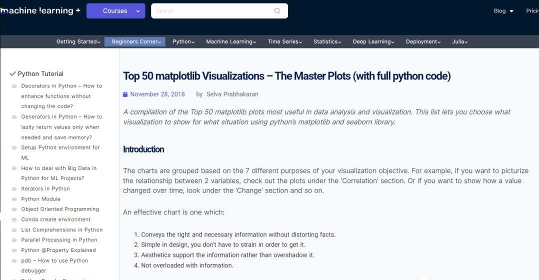
今天分享一个很好的python绘图资源: https://www.machinelearningplus.com/plots/top-50-matplotlib-visualizations-the-master-plots-python/
这个网站提供了科研论文种最常见的50种Python绘图(Matplotlib/Seaborn)方法加代码。 根据可视化目标的 7 个不同用途进行分组。例如,如果您想描绘两个变量之间的关系,请查看Correlation部分下的图表。或者,如果您想显示一个值如何随时间变化,请查看Change部分等。 本文展示部分优秀案例,完整的代码见网站,数据见后文: Correlation相关图用于可视化 2 个或多个变量之间的关系。也就是说,一个变量相对于另一个变量如何变化。 线性回归拟合了解两个变量如何相互变化,最佳拟合线是一种很好的方法 。下图显示了最佳拟合线在数据中不同组之间的差异。要禁用分组并仅为整个数据集绘制一条最佳拟合线,删除以下参数。hue='cyl'sns.lmplot() import seaborn as sns # Import Data df = pd.read_csv("./python/matplotlib-data/mpg_ggplot2.csv") df_select = df.loc[df.cyl.isin([4,8]), :] # Plot sns.set_style("white") gridobj = sns.lmplot(x="displ", y="hwy", hue="cyl", data=df_select, height=7, aspect=1.6, robust=True, palette='tab10', scatter_kws=dict(s=60, linewidths=.7, edgecolors='black')) # Decorations gridobj.set(xlim=(0.5, 7.5), ylim=(0, 50)) plt.title("Scatterplot with line of best fit grouped by number of cylinders", fontsize=20) plt.show()
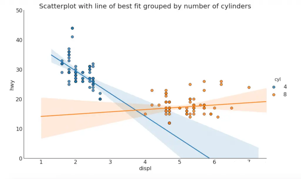
边际箱线图的用途与边际直方图类似。箱线图有助于确定 X 和 Y 的中位数、第 25 个和第 75 个百分位数。 import pandas as pd Import Datadf = pd.read_csv(“./python/matplotlib-data/mpg_ggplot2.csv”) Create Fig and gridspecfig = plt.figure(figsize=(16, 10), dpi= 80) grid = plt.GridSpec(4, 4, hspace=0.5, wspace=0.2) Define the axesax_main = fig.add_subplot(grid[:-1, :-1]) ax_right = fig.add_subplot(grid[:-1, -1], xticklabels=[], yticklabels=[]) ax_bottom = fig.add_subplot(grid[-1, 0:-1], xticklabels=[], yticklabels=[]) Scatterplot on main axax_main.scatter(‘displ’, ‘hwy’, s=df.cty*5, c=df.manufacturer.astype(‘category’).cat.codes, alpha=.9, data=df, cmap=“Set1”, edgecolors=‘black’, linewidths=.5) Add a graph in each partsns.boxplot(df.hwy, ax=ax_right, orient=“v”) sns.boxplot(df.displ, ax=ax_bottom, orient=“h”) Decorations ------------------ # Remove x axis name for the boxplot ax_bottom.set(xlabel='') ax_right.set(ylabel='') # Main Title, Xlabel and YLabel ax_main.set(title='Scatterplot with Histograms \n displ vs hwy', xlabel='displ', ylabel='hwy') # Set font size of different components ax_main.title.set_fontsize(20) for item in ([ax_main.xaxis.label, ax_main.yaxis.label] + ax_main.get_xticklabels() + ax_main.get_yticklabels()): item.set_fontsize(14) plt.show()
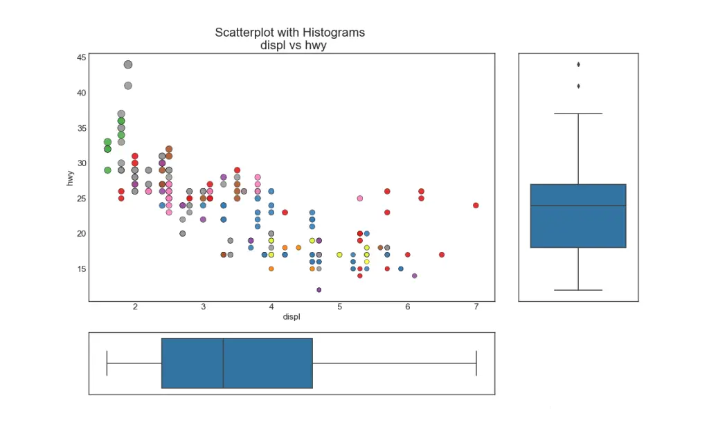
相关图用于直观地查看给定二维数组中所有可能的数字变量对之间的相关性度量。 # Import Dataset df = pd.read_csv("./python/matplotlib-data/mtcars.csv") # Plot plt.figure(figsize=(12,10), dpi= 80) sns.heatmap(df.corr(), xticklabels=df.corr().columns, yticklabels=df.corr().columns, cmap='RdYlGn', center=0, annot=True) # Decorations plt.title('Correlogram of mtcars', fontsize=22) plt.xticks(fontsize=12) plt.yticks(fontsize=12) plt.show()
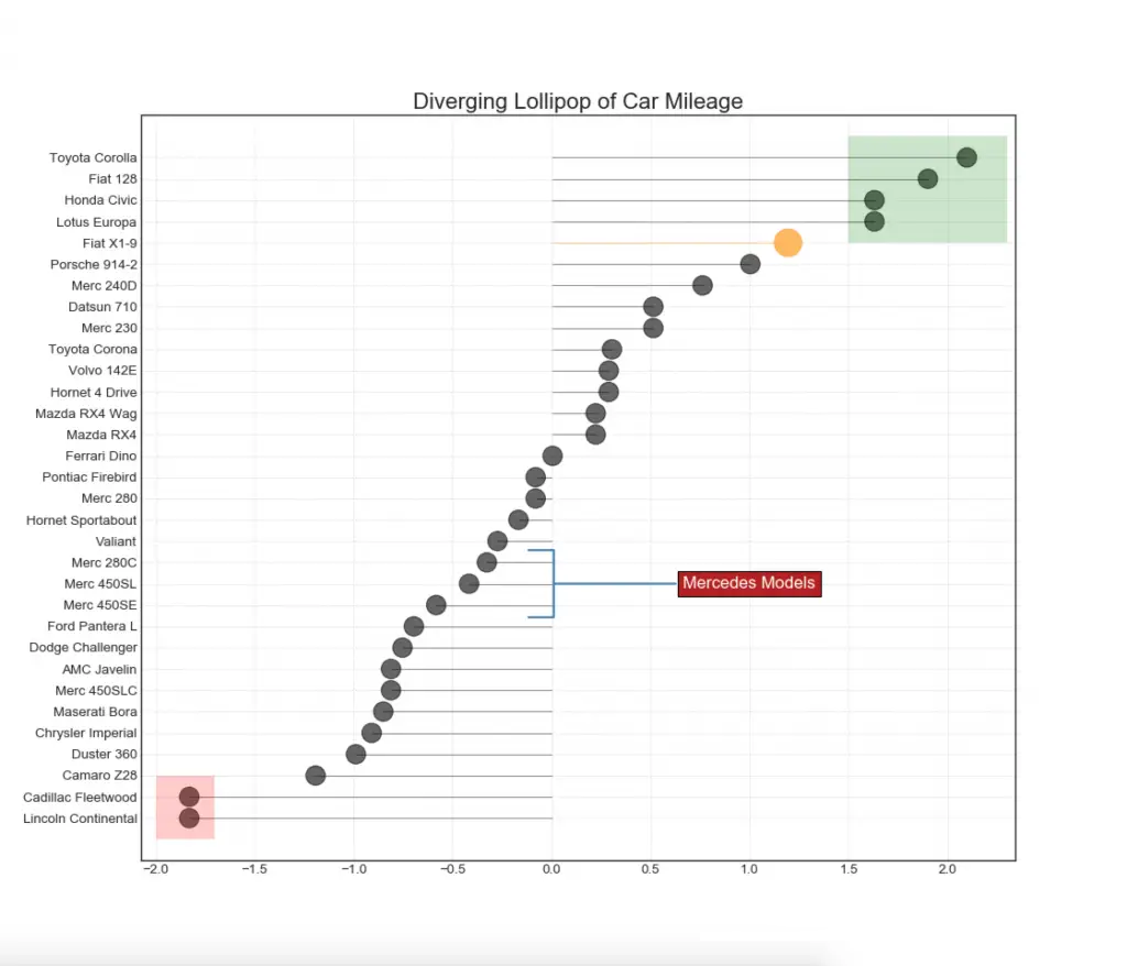
面积图是较新的图绘,建议掌握 通过为轴和线之间的区域着色,面积图不仅更加强调波峰和波谷,而且更加强调高点和低点的持续时间。高点持续时间越长,线下区域就越大。 import numpy as np import pandas as pd import matplotlib.pyplot as plt # Prepare Data df = pd.read_csv("./python/matplotlib-data/economics.csv", parse_dates=['date']).head(100) x = np.arange(df.shape[0]) y_returns = (df.psavert.diff().fillna(0)/df.psavert.shift(1)).fillna(0) * 100 # Plot plt.figure(figsize=(16,10), dpi= 80) plt.fill_between(x[1:], y_returns[1:], 0, where=y_returns[1:] >= 0, facecolor='green', interpolate=True, alpha=0.7) plt.fill_between(x[1:], y_returns[1:], 0, where=y_returns[1:] 'size':22}) ax.set(ylabel='Miles Per Gallon', ylim=(0, 30)) plt.xticks(df.index, df.manufacturer.str.upper(), rotation=60, horizontalalignment='right', fontsize=12) # Add patches to color the X axis labels p1 = patches.Rectangle((.57, -0.005), width=.33, height=.13, alpha=.1, facecolor='green', transform=fig.transFigure) p2 = patches.Rectangle((.124, -0.005), width=.446, height=.13, alpha=.1, facecolor='red', transform=fig.transFigure) fig.add_artist(p1) fig.add_artist(p2) plt.show()
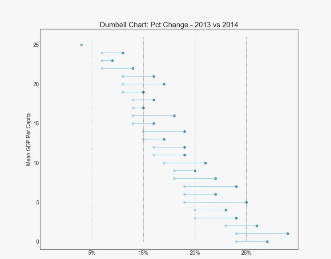
哑铃图传达了各种项目的最大最小位置以及项目的排名顺序。 import matplotlib.lines as mlines # Import Data df = pd.read_csv("./python/matplotlib-data/health.csv") df.sort_values('pct_2014', inplace=True) df.reset_index(inplace=True) # Func to draw line segment def newline(p1, p2, color='black'): ax = plt.gca() l = mlines.Line2D([p1[0],p2[0]], [p1[1],p2[1]], color='skyblue') ax.add_line(l) return l # Figure and Axes fig, ax = plt.subplots(1,1,figsize=(14,14), facecolor='#f7f7f7', dpi= 80) # Vertical Lines ax.vlines(x=.05, ymin=0, ymax=26, color='black', alpha=1, linewidth=1, linestyles='dotted') ax.vlines(x=.10, ymin=0, ymax=26, color='black', alpha=1, linewidth=1, linestyles='dotted') ax.vlines(x=.15, ymin=0, ymax=26, color='black', alpha=1, linewidth=1, linestyles='dotted') ax.vlines(x=.20, ymin=0, ymax=26, color='black', alpha=1, linewidth=1, linestyles='dotted') # Points ax.scatter(y=df['index'], x=df['pct_2013'], s=50, color='#0e668b', alpha=0.7) ax.scatter(y=df['index'], x=df['pct_2014'], s=50, color='#a3c4dc', alpha=0.7) # Line Segments for i, p1, p2 in zip(df['index'], df['pct_2013'], df['pct_2014']): newline([p1, i], [p2, i]) # Decoration ax.set_facecolor('#f7f7f7') ax.set_title("Dumbell Chart: Pct Change - 2013 vs 2014", fontdict={'size':22}) ax.set(xlim=(0,.25), ylim=(-1, 27), ylabel='Mean GDP Per Capita') ax.set_xticks([.05, .1, .15, .20]) ax.set_xticklabels(['5%', '15%', '20%', '25%']) ax.set_xticklabels(['5%', '15%', '20%', '25%']) plt.show()
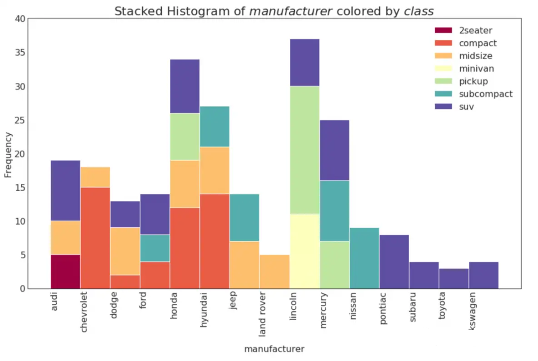
介绍多变量直方图,密度图,分布点图(较新的图绘方式) 略过了传统的箱线图、小提琴图 多变量直方图分类变量的直方图显示该变量的频率分布。通过为条形着色,将分布与另一个代表颜色的分类变量联系起来可视化。 # Import Data df = pd.read_csv("./python/matplotlib-data/mpg_ggplot2.csv") # Prepare data x_var = 'manufacturer' groupby_var = 'class' df_agg = df.loc[:, [x_var, groupby_var]].groupby(groupby_var) vals = [df[x_var].values.tolist() for i, df in df_agg] # Draw plt.figure(figsize=(16,9), dpi= 80) colors = [plt.cm.Spectral(i/float(len(vals)-1)) for i in range(len(vals))] n, bins, patches = plt.hist(vals, df[x_var].unique().__len__(), stacked=True, density=False, color=colors[:len(vals)]) # Decoration plt.legend({group:col for group, col in zip(np.unique(df[groupby_var]).tolist(), colors[:len(vals)])}) plt.title(f"Stacked Histogram of ${x_var}$ colored by ${groupby_var}$", fontsize=22) plt.xlabel(x_var) plt.ylabel("Frequency") plt.ylim(0, 40) plt.xticks(ticks=bins, labels=np.unique(df[x_var]).tolist(), rotation=90, horizontalalignment='left') plt.show()
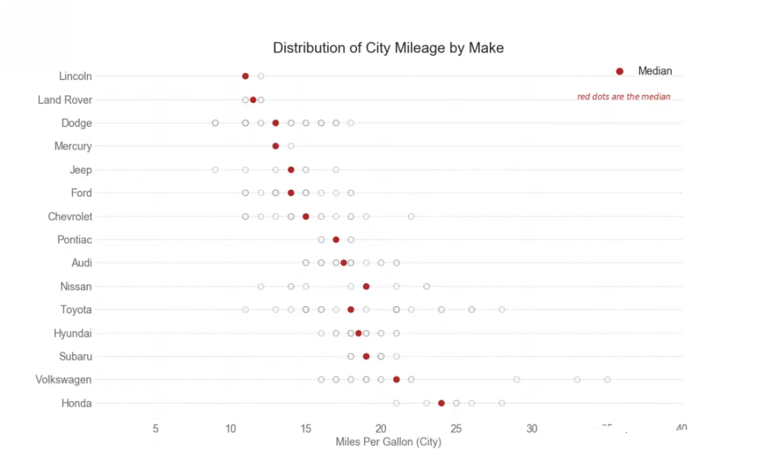
密度图是一种常用的可视化连续变量分布的工具。按类变量对它们进行分组,您可以探究各变量之间的关系和差异。 带直方图的密度曲线汇集了两个图传达的集体信息,可以将它们都放在一个图中。 # Import Data import seaborn as sns df = pd.read_csv("./python/matplotlib-data/mpg_ggplot2.csv") # Draw Plot plt.figure(figsize=(13,10), dpi= 80) sns.distplot(df.loc[df['class'] == 'compact', "cty"], color="dodgerblue", label="Compact", hist_kws={'alpha':.7}, kde_kws={'linewidth':3}) sns.distplot(df.loc[df['class'] == 'suv', "cty"], color="orange", label="SUV", hist_kws={'alpha':.7}, kde_kws={'linewidth':3}) sns.distplot(df.loc[df['class'] == 'minivan', "cty"], color="g", label="minivan", hist_kws={'alpha':.7}, kde_kws={'linewidth':3}) plt.ylim(0, 0.35) # Decoration plt.title('Density Plot of City Mileage by Vehicle Type', fontsize=22) plt.legend() plt.show() 分布式点图分布点图显示按组分割的点的单变量分布。点越暗,该区域中的数据点越集中。通过对中位数进行不同的着色,各组的真实定位立即变得一目了然。 import matplotlib.patches as mpatches # Prepare Data df_raw = pd.read_csv("./python/matplotlib-data/mpg_ggplot2.csv") cyl_colors = {4:'tab:red', 5:'tab:green', 6:'tab:blue', 8:'tab:orange'} df_raw['cyl_color'] = df_raw.cyl.map(cyl_colors) # Mean and Median city mileage by make df = df_raw[['cty', 'manufacturer']].groupby('manufacturer').apply(lambda x: x.mean()) df.sort_values('cty', ascending=False, inplace=True) df.reset_index(inplace=True) df_median = df_raw[['cty', 'manufacturer']].groupby('manufacturer').apply(lambda x: x.median()) # Draw horizontal lines fig, ax = plt.subplots(figsize=(16,10), dpi= 80) ax.hlines(y=df.index, xmin=0, xmax=40, color='gray', alpha=0.5, linewidth=.5, linestyles='dashdot') # Draw the Dots for i, make in enumerate(df.manufacturer): df_make = df_raw.loc[df_raw.manufacturer==make, :] # ax.scatter(y=np.repeat(i, df_make.shape[0]), x='cty', data=df_make, s=75, edgecolors='gray', c='w', alpha=0.5) ax.scatter(y=np.repeat(i, df_make.shape[0]), x=df_make['cty'], s=75, edgecolors='gray', c='w', alpha=0.5) ax.scatter(y=i, x='cty', data=df_median.loc[df_median.index==make, :], s=75, c='firebrick') # Annotate ax.text(33, 13, "$red \; dots \; are \; the \: median$", fontdict={'size':12}, color='firebrick') # Decorations red_patch = plt.plot([],[], marker="o", ms=10, ls="", mec=None, color='firebrick', label="Median") plt.legend(handles=red_patch) ax.set_title('Distribution of City Mileage by Make', fontdict={'size':22}) ax.set_xlabel('Miles Per Gallon (City)', alpha=0.7) ax.set_yticks(df.index) ax.set_yticklabels(df.manufacturer.str.title(), fontdict={'horizontalalignment': 'right'}, alpha=0.7) ax.set_xlim(1, 40) plt.xticks(alpha=0.7) plt.gca().spines["top"].set_visible(False) plt.gca().spines["bottom"].set_visible(False) plt.gca().spines["right"].set_visible(False) plt.gca().spines["left"].set_visible(False) plt.grid(axis='both', alpha=.4, linewidth=.1) plt.show()
介绍华夫图,树形图 省略传统的饼图 华夫图一种较新的图绘,用于展示各变量的分布 #! pip install pywaffle # Reference: https://stackoverflow.com/questions/41400136/how-to-do-waffle-charts-in-python-square-piechart from pywaffle import Waffle # Import df_raw = pd.read_csv("./python/matplotlib-data/mpg_ggplot2.csv") # Prepare Data df = df_raw.groupby('class').size().reset_index(name='counts') n_categories = df.shape[0] colors = [plt.cm.inferno_r(i/float(n_categories)) for i in range(n_categories)] # Draw Plot and Decorate fig = plt.figure( FigureClass=Waffle, plots={ 111: { 'values': df['counts'], 'labels': ["{0} ({1})".format(n[0], n[1]) for n in df[['class', 'counts']].itertuples()], 'legend': {'loc': 'upper left', 'bbox_to_anchor': (1.05, 1), 'fontsize': 12}, 'title': {'label': '# Vehicles by Class', 'loc': 'center', 'fontsize':18} }, }, rows=7, colors=colors, figsize=(16, 9) )
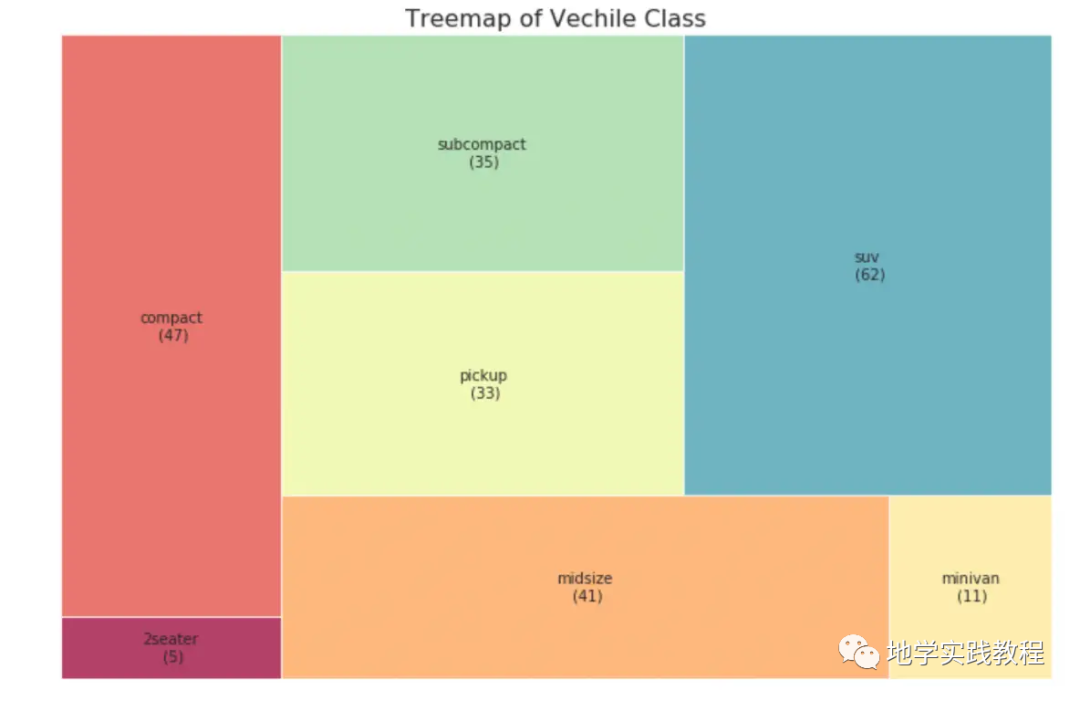
树形图类似于饼图,优点在于不误导每个组的贡献,相对于饼图更好。 # pip install squarify import squarify # Import Data df_raw = pd.read_csv("./python/matplotlib-data/mpg_ggplot2.csv") # Prepare Data df = df_raw.groupby('class').size().reset_index(name='counts') labels = df.apply(lambda x: str(x[0]) + "\n (" + str(x[1]) + ")", axis=1) sizes = df['counts'].values.tolist() colors = [plt.cm.Spectral(i/float(len(labels))) for i in range(len(labels))] # Draw Plot plt.figure(figsize=(12,8), dpi= 80) squarify.plot(sizes=sizes, label=labels, color=colors, alpha=.8) # Decorate plt.title('Treemap of Vechile Class') plt.axis('off') plt.show()
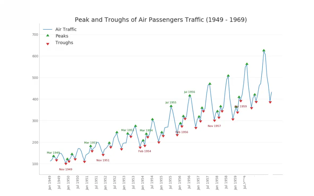
主要展示时序数据,介绍波峰波谷时间序列和双y轴时间序列 波峰波谷时间序列时间序列图用于可视化给定指标随时间的变化情况。下图可以看到 1949 年至 1969 年间航空客运量的变化情况。 # Import Data df = pd.read_csv('./python/matplotlib-data/AirPassengers.csv') # Get the Peaks and Troughs data = df['traffic'].values doublediff = np.diff(np.sign(np.diff(data))) peak_locations = np.where(doublediff == -2)[0] + 1 doublediff2 = np.diff(np.sign(np.diff(-1*data))) trough_locations = np.where(doublediff2 == -2)[0] + 1 # Draw Plot plt.figure(figsize=(16,10), dpi= 80) plt.plot('date', 'traffic', data=df, color='tab:blue', label='Air Traffic') plt.scatter(df.date[peak_locations], df.traffic[peak_locations], marker=mpl.markers.CARETUPBASE, color='tab:green', s=100, label='Peaks') plt.scatter(df.date[trough_locations], df.traffic[trough_locations], marker=mpl.markers.CARETDOWNBASE, color='tab:red', s=100, label='Troughs') # Annotate for t, p in zip(trough_locations[1::5], peak_locations[::3]): plt.text(df.date[p], df.traffic[p]+15, df.date[p], horizontalalignment='center', color='darkgreen') plt.text(df.date[t], df.traffic[t]-35, df.date[t], horizontalalignment='center', color='darkred') # Decoration plt.ylim(50,750) xtick_location = df.index.tolist()[::6] xtick_labels = df.date.tolist()[::6] plt.xticks(ticks=xtick_location, labels=xtick_labels, rotation=90, fontsize=12, alpha=.7) plt.title("Peak and Troughs of Air Passengers Traffic (1949 - 1969)", fontsize=22) plt.yticks(fontsize=12, alpha=.7) # Lighten borders plt.gca().spines["top"].set_alpha(.0) plt.gca().spines["bottom"].set_alpha(.3) plt.gca().spines["right"].set_alpha(.0) plt.gca().spines["left"].set_alpha(.3) plt.legend(loc='upper left') plt.grid(axis='y', alpha=.3) plt.show()下面的时间序列绘制了所有的波峰和波谷,并注释了选定特殊事件的发生。
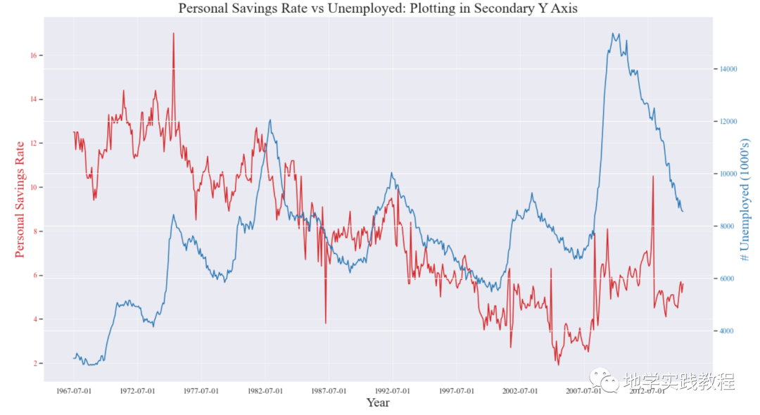
如果想显示在同一时间点测量两个不同数量的两个时间序列,可以在右侧的第二个Y轴上绘制第二个序列。 # Import Data df = pd.read_csv("./python/matplotlib-data/economics.csv") x = df['date'] y1 = df['psavert'] y2 = df['unemploy'] # Plot Line1 (Left Y Axis) fig, ax1 = plt.subplots(1,1,figsize=(16,9), dpi= 80) ax1.plot(x, y1, color='tab:red') # Plot Line2 (Right Y Axis) ax2 = ax1.twinx() # instantiate a second axes that shares the same x-axis ax2.plot(x, y2, color='tab:blue') # Decorations # ax1 (left Y axis) ax1.set_xlabel('Year', fontsize=20) ax1.tick_params(axis='x', rotation=0, labelsize=12) ax1.set_ylabel('Personal Savings Rate', color='tab:red', fontsize=20) ax1.tick_params(axis='y', rotation=0, labelcolor='tab:red' ) ax1.grid(alpha=.4) # ax2 (right Y axis) ax2.set_ylabel("# Unemployed (1000's)", color='tab:blue', fontsize=20) ax2.tick_params(axis='y', labelcolor='tab:blue') ax2.set_xticks(np.arange(0, len(x), 60)) ax2.set_xticklabels(x[::60], rotation=90, fontdict={'fontsize':10}) ax2.set_title("Personal Savings Rate vs Unemployed: Plotting in Secondary Y Axis", fontsize=22) fig.tight_layout() plt.show()
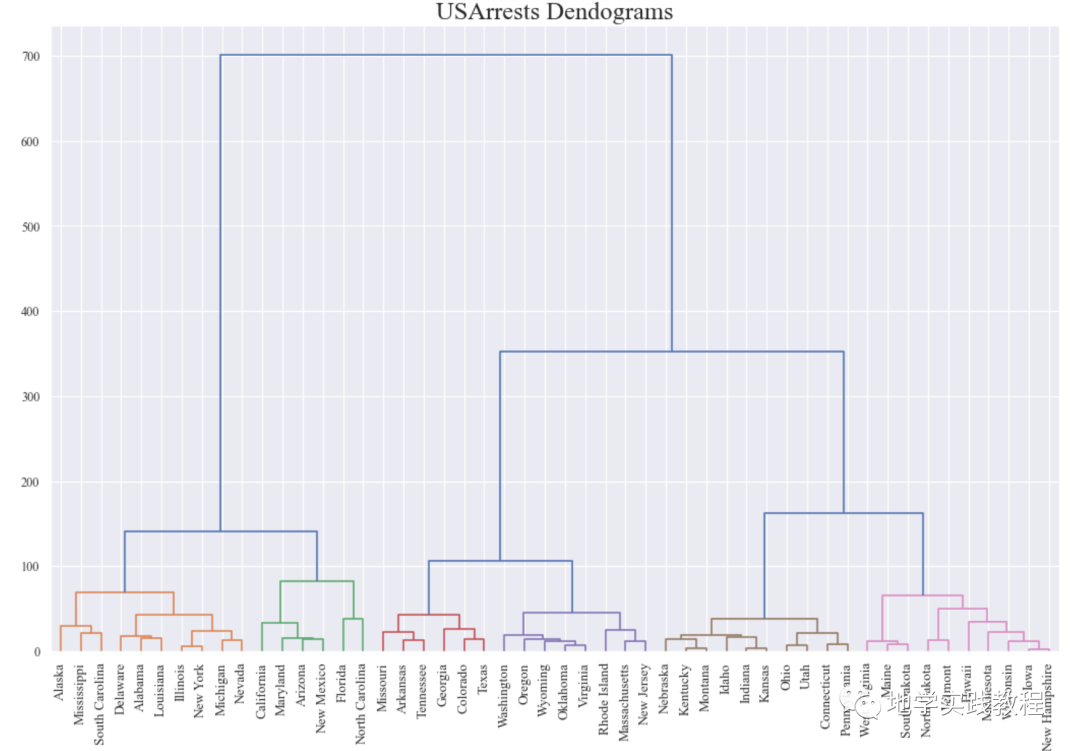
介绍树状图和聚类图 树状图 import scipy.cluster.hierarchy as shc # Import Data df = pd.read_csv('./python/matplotlib-data/USArrests.csv') # Plot plt.figure(figsize=(16, 10), dpi= 80) plt.title("USArrests Dendograms", fontsize=22) dend = shc.dendrogram(shc.linkage(df[['Murder', 'Assault', 'UrbanPop', 'Rape']], method='ward'), labels=df.State.values, color_threshold=100) plt.xticks(fontsize=12) plt.show()
聚类图可用于划分属于同一聚类的点,可以使用第一个到主成分作为 X 轴和 Y 轴。 from sklearn.cluster import AgglomerativeClustering from scipy.spatial import ConvexHull # Import Data df = pd.read_csv('./python/matplotlib-data/USArrests.csv') # Agglomerative Clustering cluster = AgglomerativeClustering(n_clusters=5, affinity='euclidean', linkage='ward') cluster.fit_predict(df[['Murder', 'Assault', 'UrbanPop', 'Rape']]) # Plot plt.figure(figsize=(14, 10), dpi= 80) plt.scatter(df.iloc[:,0], df.iloc[:,1], c=cluster.labels_, cmap='tab10') # Encircle def encircle(x,y, ax=None, **kw): if not ax: ax=plt.gca() p = np.c_[x,y] hull = ConvexHull(p) poly = plt.Polygon(p[hull.vertices,:], **kw) ax.add_patch(poly) # Draw polygon surrounding vertices encircle(df.loc[cluster.labels_ == 0, 'Murder'], df.loc[cluster.labels_ == 0, 'Assault'], ec="k", fc="gold", alpha=0.2, linewidth=0) encircle(df.loc[cluster.labels_ == 1, 'Murder'], df.loc[cluster.labels_ == 1, 'Assault'], ec="k", fc="tab:blue", alpha=0.2, linewidth=0) encircle(df.loc[cluster.labels_ == 2, 'Murder'], df.loc[cluster.labels_ == 2, 'Assault'], ec="k", fc="tab:red", alpha=0.2, linewidth=0) encircle(df.loc[cluster.labels_ == 3, 'Murder'], df.loc[cluster.labels_ == 3, 'Assault'], ec="k", fc="tab:green", alpha=0.2, linewidth=0) encircle(df.loc[cluster.labels_ == 4, 'Murder'], df.loc[cluster.labels_ == 4, 'Assault'], ec="k", fc="tab:orange", alpha=0.2, linewidth=0) # Decorations plt.xlabel('Murder'); plt.xticks(fontsize=12) plt.ylabel('Assault'); plt.yticks(fontsize=12) plt.title('Agglomerative Clustering of USArrests (5 Groups)', fontsize=22) plt.show()
本文只展示了TOP 50常见图绘中的一部分,完整代码请在网站中直接查询: https://www.machinelearningplus.com/plots/top-50-matplotlib-visualizations-the-master-plots-python/ 最后我们准备了一门非常系统的爬虫课程,除了为你提供一条清晰、无痛的学习路径,我们甄选了最实用的学习资源以及庞大的主流爬虫案例库。短时间的学习,你就能够很好地掌握爬虫这个技能,获取你想得到的数据。 01 专为0基础设置,小白也能轻松学会我们把Python的所有知识点,都穿插在了漫画里面。 在Python小课中,你可以通过漫画的方式学到知识点,难懂的专业知识瞬间变得有趣易懂。
你就像漫画的主人公一样,穿越在剧情中,通关过坎,不知不觉完成知识的学习。 02 无需自己下载安装包,提供详细安装教程
这份完整版的Python全套学习资料已经上传CSDN,朋友们如果需要也可以扫描下方csdn官方二维码或者点击主页和文章下方的微信卡片获取领取方式,【保证100%免费】 |


【本文地址】
| 今日新闻 |
| 推荐新闻 |
| 专题文章 |