excel负数显示红色

excel负数显示红色

Microsoft Excel displays negative numbers with a leading minus sign by default. It is good practice to make negative numbers easy to identify, and if you’re not content with this default, Excel provides a few different options for formatting negative numbers.

Microsoft Excel默认情况下显示带负号的负数。 优良作法是使负数易于识别，如果您不满意此默认值，则Excel提供了一些用于格式化负数的不同选项。

Excel provides a couple of built-in ways to display negative numbers, and you can also set up custom formatting. Let’s dive in.

Excel提供了两种显示负数的内置方法，您还可以设置自定义格式。 让我们潜入。

One thing to note here is that Excel will display different built-in options depending on the region and language settings in your operating system.

这里要注意的一件事是，Excel将根据操作系统中的区域和语言设置显示不同的内置选项。

For those in the US, Excel provides the following built-in options for displaying negative numbers:

对于美国的用户，Excel提供了以下内置选项来显示负数：

In the UK and many other European countries, you’ll typically be able to set negative numbers to show in black or red and with or without a minus sign (in both colors) but have no option for parentheses. You can learn more about these regional settings on Microsoft’s website.

在英国和许多其他欧洲国家/地区，您通常可以设置负数，以黑色或红色显示，并带有或不带有减号(两种颜色)，但括号中没有任何选择。 您可以在Microsoft网站上了解有关这些区域设置的更多信息。

No matter where you are, though, you’ll be able to add in additional options by customizing the number format, which we’ll cover in the next section.

不过，无论您身在何处，都可以通过自定义数字格式来添加其他选项，我们将在下一部分中介绍。

To change to a different built-in format, right-click a cell (or range of selected cells) and then click the “Format Cells” command. You can also press Ctrl+1.

要更改为其他内置格式，请右键单击一个单元格(或所选单元格的范围)，然后单击“设置单元格格式”命令。 您也可以按Ctrl + 1。

In the Format Cells window, switch to the “Number” tab. On the left, choose the “Number” category. On the right, choose an option from the “Negative Numbers” list and then hit “OK.”

在“设置单元格格式”窗口中，切换到“数字”选项卡。 在左侧，选择“数字”类别。 在右侧，从“负数”列表中选择一个选项，然后单击“确定”。

Note that the image below shows the options you’d see in the US. We will be talking about creating your own custom formats in the next section, so it’s no problem if what you want is not shown.

请注意，下图显示了在美国看到的选项。 在下一节中，我们将讨论如何创建自己的自定义格式，因此，如果没有显示您想要的内容，这没问题。

Here, we’ve chosen to display negative values in red with parentheses.

在这里，我们选择以红色显示带有括号的负值。

This display is much more identifiable than the Excel default.

此显示比Excel默认值更容易识别。

You can also create your own number formats in Excel. This provides you with the ultimate control over how the data is displayed.

您也可以在Excel中创建自己的数字格式。 这使您可以最终控制数据的显示方式。

Start by right-clicking a cell (or range of selected cells) and then clicking the “Format Cells” command. You can also press Ctrl+1.

首先右键单击一个单元格(或选定单元格的范围)，然后单击“设置单元格格式”命令。 您也可以按Ctrl + 1。

On the “Number” tab, select the “Custom” category on the left.

在“数字”选项卡上，选择左侧的“自定义”类别。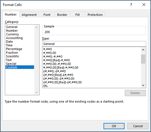

You’ll see a list of different custom formats on the right. This can seem a little confusing at first but is nothing to fear.

您会在右侧看到不同自定义格式的列表。 乍一看，这似乎有点令人困惑，但不必担心。

Each custom format is split into up to four sections, with each section separated by a semi-colon.

每个自定义格式最多可分为四个部分，每个部分之间用分号分隔。

The first section is for positive values, the second for negatives, the third for zero values, and the last section for text. You do not have to have all sections in a format.

第一部分用于正值，第二部分用于负数，第三部分用于零值，最后一部分用于文本。 您不必使所有部分都采用某种格式。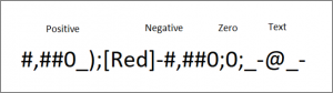

As an example, let’s create a negative number format which includes all of the below.

例如，让我们创建一个包含以下所有内容的负数格式。

In the Type box, enter the code below.

在“类型”框中，输入以下代码。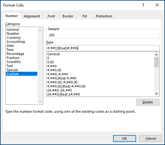

Each symbol has a meaning, and in this format, the # represents the display of a significant digit, and the 0 is the display of an insignificant digit. This negative number is enclosed in parenthesis and also displayed in blue. There are 57 different colors you can specify by name or number in a custom number format rule. Remember that the semi-colon separates the positive and negative number display.

每个符号都有含义，在此格式中，＃表示有效数字显示，0表示无效数字显示。 该负数用括号括起来，并用蓝色显示。 您可以在自定义数字格式规则中通过名称或数字指定57种不同的颜色。 请记住，分号分隔了正数和负数显示。

And here’s our result:

这是我们的结果：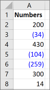

Custom formatting is a useful Excel skill to have. You can take formatting beyond the standard settings provided in Excel that may not be sufficient for your needs. Formatting negative numbers is one of the most common uses of this tool.

自定义格式是一项有用的Excel技能。 您可以采取超出Excel中提供的标准设置的格式，而这可能不足以满足您的需求。 格式化负数是此工具最常见的用途之一。

翻译自: https://www.howtogeek.com/401522/how-to-change-how-excel-displays-negative-numbers/

excel负数显示红色