| 图像边缘检测 | 您所在的位置:网站首页 › 边缘检测意义 › 图像边缘检测 |
图像边缘检测
|
文章目录
前言一、图像边缘检测二、边缘检测算子1. Roberts算子2. Prewitt算子3. Sobel算子
三、代码实现总结
前言
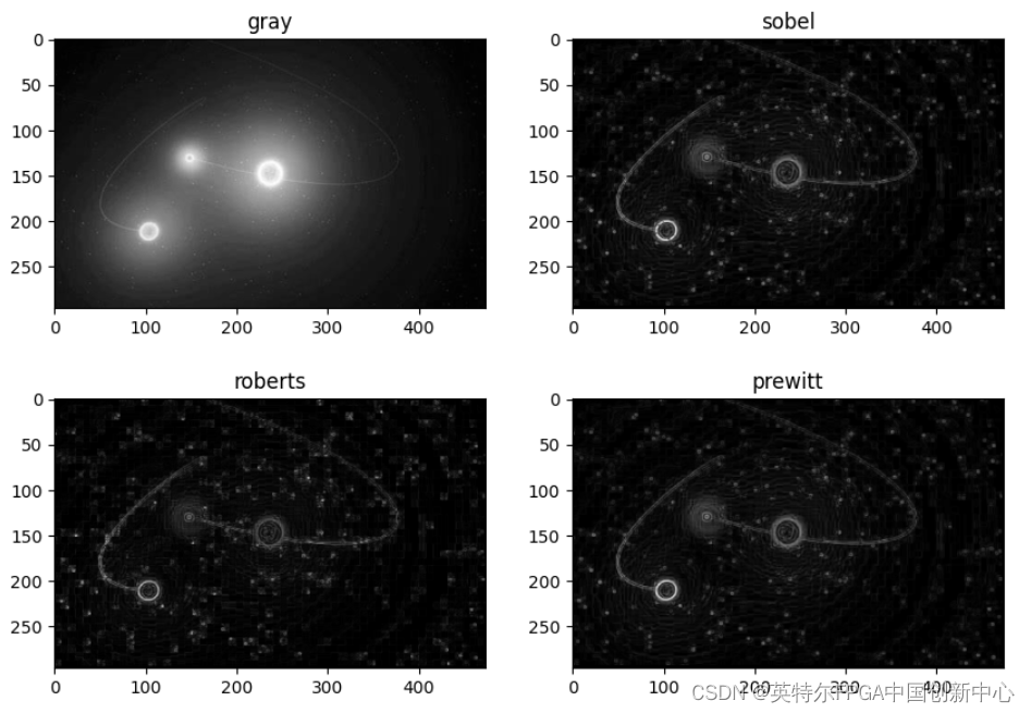
有了图像放大缩小,图像灰度化处理等相关基础知识过后,就可以进行图像边缘检测了。边缘检测最后也会在FPGA上面实现,此处小编已经控制不住要剧透了。也是一样,先从软件的角度来理解这些图像边缘检测算法。 一、图像边缘检测 边缘检测原理如下动态图所示。假如你有一些别人发明的算子,算子在第二章介绍。使用算子在原图上进行扫描,算子中的值乘以对应的像素值,然后加起来就行了。你可以使用截图工具,截取动态图,计算一下是否正确。 算子其实就是滤波器,在深度学习里面又叫卷积,下面3种算子给出了具体的值,而在卷积神经网络里面,卷积核的值是需要训练得到。 1. Roberts算子G x = [ 1 0 0 − 1 ] G y = [ 0 − 1 1 0 ] G_x = \begin{bmatrix} 1 & 0 \\ 0 & -1 \end{bmatrix} \quad\quad\quad G_y = \begin{bmatrix} 0 & -1 \\ 1 & 0 \end{bmatrix} Gx=[100−1]Gy=[01−10] 2. Prewitt算子G x = [ − 1 0 1 − 1 0 1 − 1 0 1 ] G y = [ − 1 − 1 − 1 0 0 0 1 1 1 ] G_x = \begin{bmatrix} -1 & 0 & 1\\ -1 & 0 & 1\\ -1 & 0 & 1 \end{bmatrix} \quad\quad\quad G_y = \begin{bmatrix} -1 & -1 & -1\\ 0 & 0 & 0\\ 1 & 1 & 1 \end{bmatrix} Gx= −1−1−1000111 Gy= −101−101−101 3. Sobel算子G x = [ − 1 0 + 1 − 2 0 + 2 − 1 0 + 1 ] G y = [ + 1 + 2 + 1 0 0 0 − 1 − 2 1 ] G_x = \begin{bmatrix} -1 & 0 & +1\\ -2 & 0 & +2\\ -1 & 0 & +1 \end{bmatrix} \quad\quad\quad G_y = \begin{bmatrix} +1 & +2 & +1\\ 0 & 0 & 0\\ -1 & -2 & 1 \end{bmatrix} Gx= −1−2−1000+1+2+1 Gy= +10−1+20−2+101 三、代码实现 # robert算子 robert_x = np.array([[1, 0], [0, -1]]) robert_y = np.array([[0, -1], [1, 0]]) # prewitt算子 prewitt_x = np.array([[-1, 0, 1], [-1, 0, 1], [-1, 0, 1]]) prewitt_y = np.array([[1, 1, 1], [0, 0, 0], [-1, -1, -1]]) # sobel算子 sobel_x = np.array([[-1, 0, +1], [-2, 0, +2], [-1, 0, +1]]) sobel_y = np.array([[+1, +2, +1], [0, 0, 0], [-1, -2, -1]]) # 图像灰度处理 def weight_gray(image): weight_image = image[:, :, 0] * 0.11 + image[:, :, 1] * 0.59 + image[:, :, 2] * 0.3 weight_image = weight_image.astype(np.uint8) return weight_image # 图像边缘检测 def edge_dimage(image, operator): shape = image.shape h, w = shape sh, sw = operator[0].shape sobel_image = np.zeros(image.shape) for i in range(h - sh): for j in range(w - sw): ix = np.multiply(image[i: i + sh, j: j + sw], operator[0]) iy = np.multiply(image[i: i + sh, j: j + sw], operator[1]) ix = np.sum(ix) iy = np.sum(iy) ig = np.sqrt(ix ** 2 + iy ** 2) sobel_image[i, j] = ig sobel_image = sobel_image.astype(np.uint8) return sobel_image image = cv2.imread("three_body.jpg") gray = weight_gray(image) roimage = edge_dimage(gray, (robert_x, robert_y)) primage = edge_dimage(gray, (prewitt_x, prewitt_y)) sbimage = edge_dimage(gray, (sobel_x, sobel_y)) # 画子图 plt.figure(figsize=(10, 7)) plt.subplot(221) plt.title("gray") plt.imshow(gray, cmap='gray') plt.subplot(222) plt.title("sobel") plt.imshow(sbimage, cmap='gray') plt.subplot(223) plt.title("roberts") plt.imshow(roimage, cmap='gray') plt.subplot(224) plt.title("prewitt") plt.imshow(primage, cmap='gray')
这大概就是卷积神经网络的由来,以前叫做算子,现在叫做卷积。小编也迫不及待的想要动手实现卷积神经网络了(numpy),敬请期待。 |

【本文地址】