| 索伯(Sobel)算子原理讲解和实现 | 您所在的位置:网站首页 › sobel算子的推导 › 索伯(Sobel)算子原理讲解和实现 |
索伯(Sobel)算子原理讲解和实现
|
文章结构
1. 简述Sobel算子2. ndimage.Sobel3. Sobel 算子自实现4. Sobel算子的一些缺陷和替代方案
1. 简述Sobel算子
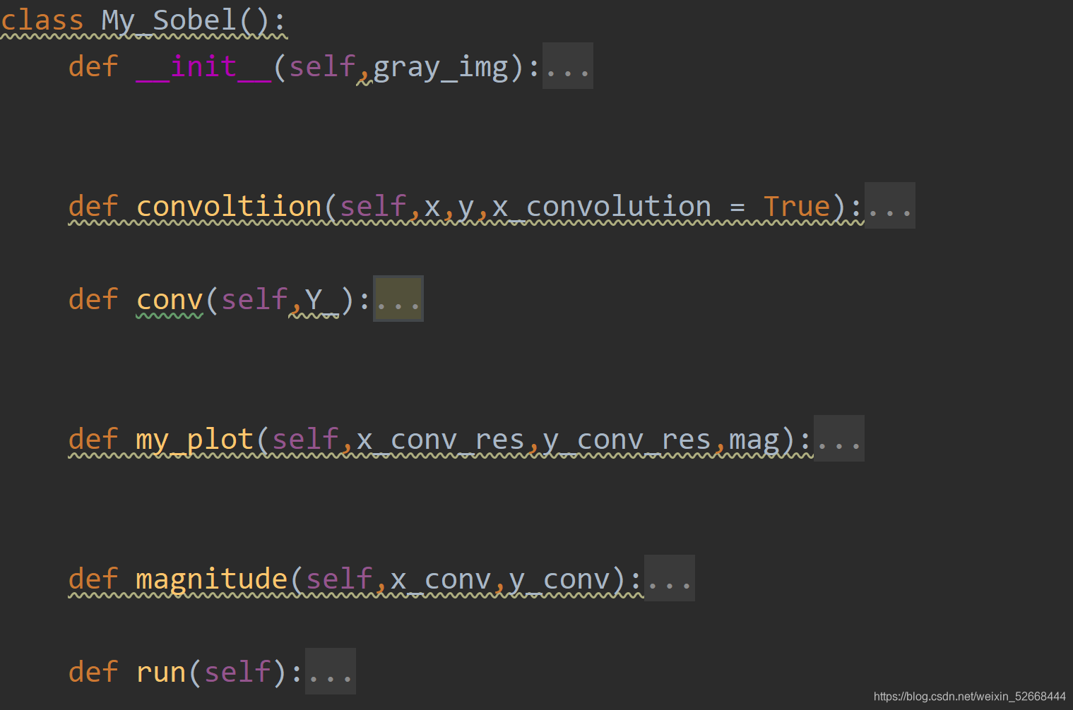
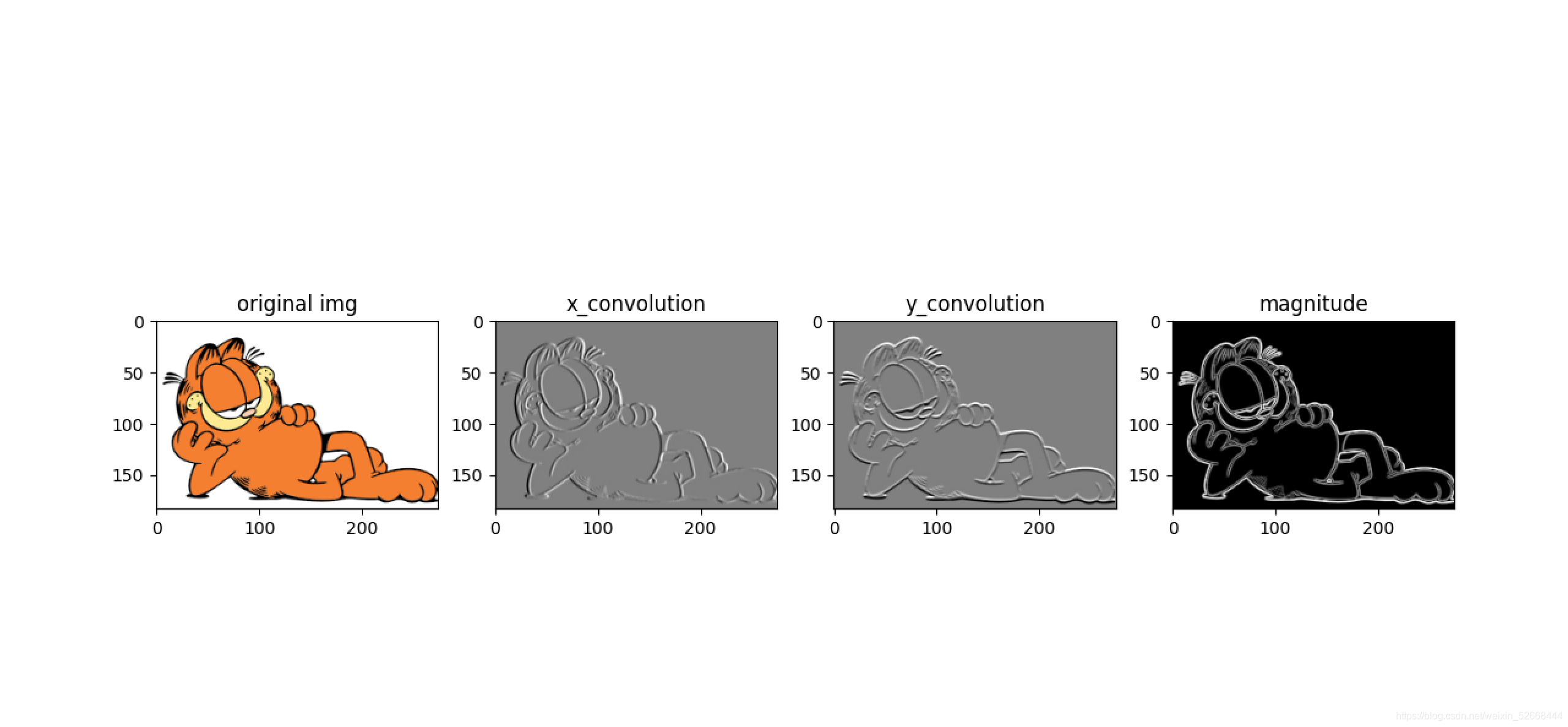
索伯算子主要用于边界检测,该算法相对其他的边界检测算法而言是比较的容易。但是对于噪声的鲁棒性要低于其他的边界检测技术。比如canny。 索伯算子是一种多用于边缘检测的离散性差分算子。索伯算子有两组不同的卷积因子,可以为一张图片做横向以及纵向的平面卷积。详细的讲就是,假设要对一张图中的(x,y)这个像素使用索伯算子。首先用两个卷积因子分别对该点做卷积,从而可得出该点在这两个方向上的亮度差分近似值。将xy两个方向的亮度近似值进行结合之后,即可得到该点亮度。 得到的是一个数,如果这个值大于了阈值,那么这个点就可以被考虑成边缘点。 2. ndimage.Sobel首先看看ndimage提供的索伯算子是什么样的效果。要注意的是 python中提供的sobel API,有的只能支出2维的输入,如果不降图片变成灰度图片,直接使用API会出现报错。 ValueError: The parameter `image` must be a 2-dimensional arraysobel算子的实现主要分以下几步来完成。 首先需要将需要边缘检测的图像进行黑白处理。因为色彩对于边缘检测的影响很小。 分别计算灰度图片横向和纵向的梯度。 计算两个方向梯度的幅值。 规范化梯度 下面以一张彩色的加菲猫照片,来展示简单边缘检测的基本流程个效果。 代码分成两个板块:边缘检测和图像展示 边缘检测的代码展示如下: def edges_detection(img): #img must be grayscaled img_gray = sc.rgb2gray(img) #partial derivative of x_axis dx = ndimage.sobel(img_gray,1) dy = ndimage.sobel(img_gray,0) #magnitude mag = np.hypot(dx,dy) #shown as image. must be 8 bit integer # mag = 255.0/ np.amax(mag) # mag = mag.astype(np.int8) return mag原图以及图像结果的展示的代码如下所示: def plot_res(img,mag): figure = plt.figure() figure.add_subplot(121) plt.imshow(img) # plt.show() figure.add_subplot(122) plt.imshow(mag) plt.show()结果展示如图所示: 以下内容为sobel算子python自实现的一些细节。下图是sobel算子实现需要的一些函数 convolution函数的是用于对某一个像素点(x,y)进行横向或者纵向的平面卷积。他需要3个参数,x,y,以及x_convolution。x和y顾名思义就是,当前像素的坐标,x_convolution是一个布尔值,如果为正将使用水平方向的卷积因子,反之,则使用纵向的卷积因子。 convolution 完整代码如下: def convoltiion(self,x,y,x_convolution = True): #calculate single pixel. ''' note that all operations must be done within the range. Therefore, pay attention on those pixels on the margin. operation does not start at(0,0) but (1,1), ends at(x-1,y-1). :param x: :param y: :return: ''' y_coordinate = [y-1,y,y+1] x_coordinate = [x-1,x,x+1] res = 0 if x_convolution: kernel = self.x_kernel conv_res = self.x_conv_res else: kernel = self.y_kernel conv_res = self.y_conv_res for x_k_cor_ ,x_y in zip(range(kernel.shape[1]),y_coordinate): # y = 0 ,1 2 for x_k_cor, x_x in zip(range(kernel.shape[0]),x_coordinate): # x = 0,1,2 res = res + self.gray_img[x_x,x_y] * kernel[x_k_cor,x_k_cor_] conv_res[x,y] = res return conv_res上述代码的为题在于,循环图中的每一个像素,势必不能保证算法的时间复杂度。因为图片越大,复杂度越大。 接下来需要将图片中所有的点都用上述的方法,从水平和纵向进分别进行平面卷积, 两个方向的卷积,原理上没有很大的变化,只是卷积因子发生了改变。 def conv(self,Y_): for y_coordinate in range(1,img_gray.shape[1]-1): for x_coordinate in range(1,img_gray.shape[0]-1): res_ = self.convoltiion(x_coordinate,y_coordinate,x_convolution=Y_) return res_当求得了水平方向和纵向的卷积结果之后,将两个方向的结果结合起来便可以得到赋值。 def magnitude(self,x_conv,y_conv): return np.sqrt(np.square(x_conv)+np.square(y_conv))之后显示一下效果: def my_plot(self,x_conv_res,y_conv_res,mag): figure_ = plt.figure() ax1 = figure_.add_subplot(141) ax1.set_title('original img') plt.imshow(img_array) ax2= figure_.add_subplot(142) ax2.set_title('x_convolution') plt.imshow(x_conv_res,cmap='gray') ax3 = figure_.add_subplot(143) ax3.set_title('y_convolution') plt.imshow(y_conv_res,cmap='gray') ax4 = figure_.add_subplot(144) ax4.set_title('magnitude') plt.imshow(mag,cmap='gray') plt.show()
从图中可以看到的是用sobel的边缘检测,检测出来的边界是比较粗的,意味着这样的检测方式在一些情况下是不够精确的,因为我们最理想的状态是边缘的宽度是一很窄的线(单像素),而不是一个区域。在实际的生产中,我们通常会使用canny的边缘检测算法。它的效果相符于前者的效果更好。简单而言,canny对噪音的鲁棒性要比sobel要好。 canny的API在skimage.feature中提供。代码与三者比较如下所示: canny_ = canny(img_gray, sigma=5)
|

 实现的效果与ndimage的效果类似。颜色的不同是因为在画图的时候,更改了cmap。
【本文地址】